Glossary.

GLOSSARY

Accuracy: truthfulness and certainly of a value.

Approximation: Estimation or inexact representation of a value. An approximation is a quantity that represents a desider value.

Analytical solution: Mathematical exppression that represent a system. Gives a real result. 


Gauss: Carl Friedrich Gauss. (1777-1885) German scientist and mathematician. He studied numerical methods, statistics, geometry, physics, astronomy, optics, and others.

Mathematical Model: formulation that expresses a physical phenomena or system in mathematical terms. 

Method:technic for doing something.

Numerical method: “techniques by which mathematical problems are formulated so that they can be solved with arithmetic operations.” Steven Chapra

Numerical solution: Approximation  to the result of a system.

  

Parameters: compounds of a model.

Significant digits: digit(s) that gives confidence to a number.

Total numerical error: is the summation of the truncation and round-off error.

Truncation error: “is the discrepancy introduced but the fact that numerical methods may employ approximations to represent exact mathematical operations and quantities” Steven Chapra

Vector: Vertical arrengement of numbers. It represents a serie of values.

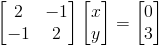
Jacobi and Gauss Seidel Method

Jacobbi

We start with a normal equation system, we represent it like a matrix, check this out:

Lets see the steps to carry out Jacobi method.

In this way we can make iterations to get real values of X.

Gauss Seidel Method:

Here we have a better version of Jacobi, we have the same process but now we use values calculate in the same iteration, fot this reason we can say Gauss Seidel Method is faster than Jacobi method!

LU Descomposition

LU descomposition

To understand LU descomposition you have to check this out:

To use LU elimination:

1- Find "L" and "U": Lower and Upper matrices.

2- You know" L" and "b", so you can get "y"

3- With "U" and "y" find "X"!

Lets see same excercise we've worked before:

A 

Step 1

To find L and U matrices:

L
U
 Step 2:
With L and b find y

Step 3:

With U and y find X

      Now you have the answer! 

Gauss Jordan Elimination

Gauss Jordan elimination

Its a new version of Gaussian elimination, which puts zeros till we have an diagonal matrix. 

Solving linear equations this method we obtain:

-->The solution of the equations. 
-->The matrix inverse.

Are you wondering the difference between Gauss Jordan and Gaussian elimination?

The difference is "Back substitution" the idea is to take a diagonal matrix and operate it on reverse order.

At the end we will have the rows of the matrix in echelon form, the diagonal will have ones and in the right side the solution vector. 

For instance:

Let's see example showed in Gaussian Elimination.

Written like a matrix:

 

At this point we have the upper triangular matrix: 

Next step is "BACK SUBSTITUTION". At the end we will get the matrix in the next form:

Inmediatly we can note that:

X = 3

Y = 1

Z = 2

                                                                                                                                                                                                                            

Gaussian elimination

Gaussian elimination

We can solve linear equation systems, or matrices of the form:

 Ax=B

Or,

If you want you can use the matrix in extended form:

You have to use elementary row operations till the matrix will be an upper triangular, like this:

At this moment we can solve the first unknown value, and using following expression we can obtain all of them:

                                                        

For instance, we have following linear equations system: 

Lets write it like a matrix:

Applying Gaussian Elimination we have: 

Its a upper triangular matrix, here we know that:

Z = 2

Going back we can obtain X and Y values, because:

Y - 5Z = -9

Solving for Y:

Y=1

Next step is find X:

X + Y + 2Z = 8

where, 

X=3

Matrices

Matrices

A matrix is a rectangular arrangement of numbers. In a matrix you will find numers in rows and columns that express linear system equations.

Source: http://www.catonmat.net/blog/wp-content/uploads/2009/11/matrix-form-two-equations.gif

If we want to solve systems of equations we must consider that:

We want to find values of x and y that make both equations true!

We can make following row transformations: 

1. Interchange rows.

2. Multiply all elements of any row by the same number (nonzero).

3. Add to all elements of a row a multiple of the corresponding elements of another row.

To solve a linear equation system we do row transformations till we obtein a matrix in its triangular form, like:

1 a b c d

0 1 e f g

0 0 1 h i

0 0 0 1 j

0 0 0 0 1

We have different types of martices, check this out:

We have a tool to know if a matrix has solutions or not: the determinant.
Lets see how to obtain the determinant of a matrix:
if we have two equations:
ax+by=c
dx+ey=f
The determinant will be:

Note that we have two lines, and the slopes will be -a/b and -d/e, for this reason if the determinant is zero, we know the lines are identicals because the slopes are equal! What does it means? We have an infinite number of solutions! 

In the other hand, if the determinant is nonzero we have different lines and there is an intersect in one point.

Example:



The determinant for this case will be: (2)(2)-(-1)(-1)=3
We know this system have a solution.

Methods

Here we have a graph that summarize methods to solve linear equations:

Secant method

SECANT METHOD

Secant method defines a line that pass through (X_n-1 , f(X_n-1)).

Similarly the other methods, we obtain next approximation with a mathematical formulation, check this out:

This formulation comes from central approximation of a function.

To carry out secant method we need two initial approximations, root could not be between this interval; for this reason this methods isn’t a bracketing method.

Here we have steps to apply secant method:

You should repeat those steps till you reach the tolerance expected each case.

Newton Raphson Method

NEWTON RAPHSON

If we want to find r, the root of a function f(x), we start with X₀ an estimate of r. From X₀ we produce an estimate X₁ , this is a improve value of the root. 

 From X₁ we can produce an estimate X₂ which is a improve value of the root. 

In this way we are going to reach an approximation close to r. 

Next dias gram shows steps to obtain an approximation using Newton Raphson Method:

Source: http://www.polyvore.com/cgi/img-set?.out=jpg&id=CiLA-pZS3hGf6J_BzGWFag&size=l

Bisection Method

 Bisection method

Consider the equation f(x) continuous in [x₁ , x₂ ], we evaluate Xm, the midpoint of the interval.

Xm = (X1+X2)/ 2

For example: 

Source: http://www.ita.uni-heidelberg.de/~banerjee/teaching/UKNum/Lecture_03.pdf

 We have two options:

• 1.       If f(x₁) and f(x_m) have opposite signs then we can reduce the range, now instead of  [x₁ , x₂ ] new interval is  [x₁ , x_m ].
• 2.       If f(x_m) and f(x₂) have opposite signs then we can reduce the range, now instead of  [x₁ , x₂ ] new interval is  [x_m , x₂ ].

We can be sure that within these values is the real root because if the function is continuous it must be zero between the selected values.

We have different possible cases working with bisection methods:

Examples:

Case 1

Case 2

 Case 3

Case 4

Source: http://www.ita.uni-heidelberg.de/~banerjee/teaching/UKNum/Lecture_03.pdf

Advantages & disadvantages of bisection method!

Chris Madden Cartoon